Hands-on GNURadio Companion

As I mentioned in my previous article, I started to explore a whole new field of software defined radios (SDRs) which I came across about a month ago. Initially it started as a requirement of learning digital signal processing (DSP) which is definitely important in my research works. While going through DSP stuff, I came across this wonderful world of SDRs and now I'm taking baby steps into the SDR world. When using SDR hardware tools, the knowledge of SDR software such as GNURadio is inevitable. GNURadio is an opensource software defined radio tool set that is being widely used by the people in this domain. The purpose of this article is to note down some of the basic stuff I learned today about using GNURadio to process signals.

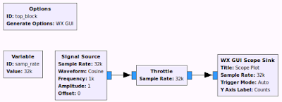
Before everything, we need GNURadio software environment up and running in my system. To avoid the installation hassles, I prefer booting my system using a USB drive with a live Linux image which are readily available from here. GNURadio software tools are pre-installed in such Linux images to make our lives easier. After booting the system with GNURadio, we can launch GNURadio Companion (GRC) tool which provide facility to visually create flow graphs that consists of different blocks. These blocks can be either signal sources, signal sink or signal processing components. An important thing to check after starting GRC for the first time is double-clicking on the 'Options' block and going to the 'General Options' field which should be set to 'WX GUI'. Setting it to some other thing from the drop down list can cause various run-time problems which I had to learn in the hard way. After setting this option, we are ready to start our adventure.

Figure - 1

Figure - 2

As our first exercise, we generate a signal and visualize it with various plots available in GNURadio. Drag and drop the relevant components from right-hand side list and create a flow graph like the one shown in Figure-1. This flow graph can be downloaded from here too. Signal Source block is used to generate the signal we want. Double-click on it and see how its settings are placed. The task of the throttle block is to control the rate of samples flowing through the flow graph. 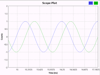The last block in the flow graph WX GUI Scope Sink draws a graph which will show us the waveform of the generated signal. Clicking on the play button on the tool bar cause the flow graph to be compiled and generate a python script. Then this python script will start to run automatically. The resulting Scope plot window is shown in Figure-2

Figure - 3

Figure - 4

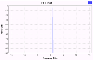
After looking at the waveform, now let's draw an FFT plot for the signals generated using Signal Source. For that, we should delete the previous sink and add a WX GUI FFT Sink block. This new flow graph is shown in Figure-3 and the source file for this new flow graph can be found here. It is important to double-click on this FFT block and look at how it's configurations are made in order to make it work. When we run this flow graph,  the FFT block will show up which has frequency in it's x-axis as shown in figure-4. Y-axis of the graph shows the power of each frequency component in dB units. As our signal source is set to 1kHz, FFT plot shows a peak at that frequency.

Figure - 5

Figure - 6

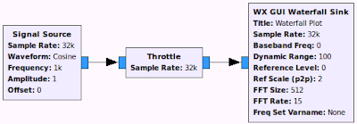
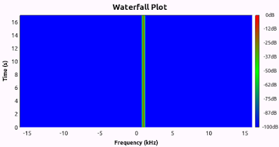
Now we explored two types of plots to visualize our signals from the source block. It's time to learn another kind of plot that is WX GUI Waterfall Sink block. It works like a spectrogram showing the power variation of various frequency components over time. Remove the previous sink block and add such a sink block in to the place as shown in figure-5. A configuration file for such a flow graph can be found here. When we run this flow graph, it shows a beautiful plot which update over time as depicted in figure-6. Among all the other plot types, I like these Waterfall plots so much since it provides a lot of information about the signals being watched.

Figure - 7

Figure - 8

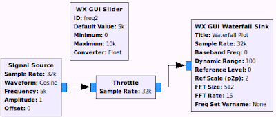
As the last thing I share in this article, let's look at how we can dynamically adjust a specific parameter in the flow graph while it is running. For this purpose, we need to employ a WX GUI Slider block. For the ID field of this block, we put a name freq2 and then in the signal source block, we should set frequency field to freq2 variable. 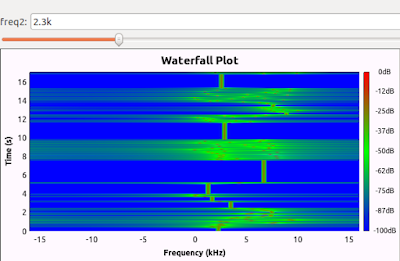Such a setting is shown in figure-7 and a suitable configuration file for such a flow graph can be found in here. When we run this flow graph, we get a waterfall plot together with a slider which can be adjusted to change the frequency of the signals generated from the source block as shown in figure-8. 

That's all for this first article about using GNURadio. I will write a few more articles with various other things I learn in GNURadio territory. Cheers!!