Biography of John Nash

Among various interesting places in UCD, I find the James Joyce library as a special place as I always admire good books. During my second visit to the library, I accidentally came across an interesting book which grabbed my attention. It's the biography of the famous mathematician John Forbes Nash written by Sylvia Nasar. The name of the book is "A Beautiful Mind" which is a famous name due to the famous movie with the same name and is based on this very same book. I had already watched the movie a few years ago and immediately felt that I should read the book too.

John Nash is an American mathematician who is famous for his contributions to Economics including Nash Equilibrium. He won the 1994 Nobel Prize in Economics. He suffered from a mental illness called Schizophrenia which caused him to see delusions and hear voices which were non-existent. His illness failed him to recognize reality and his own imaginations. His life story is so painful as he bounced between the reality and his delusions affecting his academic career and family life. He luckily had a wonderful group of people around him who never gave up with him till the end.

I learned so many things from the book about the life of this mathematician which were not represented in the movie. Of course, it is natural that when a movie is based on a book, so many details from the book has to be omitted from the book in order to fit the story into a short video. However, missing these details from the John Nash's life story makes it so incomplete. Therefore, I'm glad that I found the book.

Among so many things, I thought it is worth highlighting some interesting facts about this interesting man which I couldn't find in the movie. Let's start with some dark aspects.

(1) The movie tells us how Nash found Alicia, how they fall in love and build their family. The missing piece is that Nash had a love life before meeting Alicia. For a while,  Nash lived together with a girl called Eleanor and they had a son too. After their son was born, Nash refused to marry Eleanor and even refused to pay for the child support when she tried to take legal action. Nash's mother tried so hard to prevent her son from doing this terrible mistake but she failed. Nash later met a student called Alicia and got married to her. Eleanor even went to meet Alicia to prevent this marriage but still, Alicia didn't care.

(2) During the time when Nash was working for a defense research institution, he was arrested by police once with the charges of "indecent exposure" in a men's bathroom. Due to this incident, his security clearance was canceled making him unable to work on defense projects. It is still not clear whether Nash was gay. At some points, while he was a Ph.D. student, his behavior indicates like he had some kind of affection for male students. However, still, it is difficult to confirm.

(3) During the Korean wartime, US Government drafted young American men to go to war. Nash was on the list of compulsory military draft and it was clear that he has to join military very soon. He used his personal and family connections to remove his name from the list while some of his unfortunate Princeton colleagues had to go to war. Just imagine how many brilliant young men the war must have taken away. The move taken by Nash spared his life even though the way he did it was not right. 

(4) Nash was so determined to win a mathematical prize somehow and for that, he was supposed to publish in an American journal. He first submitted his paper to Acta Mathematica, a prestigious Swedish mathematical journal and right after getting the acceptance with comments, he immediately withdrew the paper and submitted to American Journal of Mathematics. Swedish reviewers were so outraged by Nash's unprofessional behavior.

Having said so many negative aspects of this brilliant man, I still find amazing things in this person. Among so many other things, this is the most fascinating thing about John Nash. Even though he was suffering from the mental illness called Schizophrenia, which caused him to see delusions and hear voices, he believed in something which is even sane people fail to recognize as a wonderful idea.

Nash believed that there is an incoming Alien Invasion to the Earth. He thought that he can figure out how the Aliens are going to do it by decoding secret messages. His idea was that the whole world should unite and fight back. He tried to convince his fellows, high profile members of the government and many others about this invasion but nobody believed him. Being unable to convince others, finally, he left the US and traveled to Switzerland. There he visited the US embassy in Switzerland and attempted to rip off his passport in front of the officials. He said that he no longer an American citizen but a World Citizen. Although this idea was never accepted and he was deported back to the US, I find this an awesome idea.

Do we have to be insane to think that these divisions among human race are not going to help us in any way?

~**********~

Diving into FAT file system with a Hex Editor

In this post, I'm going to explore a disk image which contains a FAT32 partition completely using a hex editor. This exploration provides an important insight on how FAT file system works. The disk image I'm using for this is a 100MB long file which can be download from here. SHA1 hash value of the file is as follows.

d665dd4454f9b7fc91852d1ac8eb01a8f42ed6be

(1) First of all, we open this disk image using Okteta. Here's the first 512 bytes which is the first sector of the disk looks like. That means this is the Master Boot Record (MBR). We can see distinguishable features of the MBR here. The very first thing to spot is that the last two bytes located at the offset 0x01FE of this sector contains the value 0x55AA.

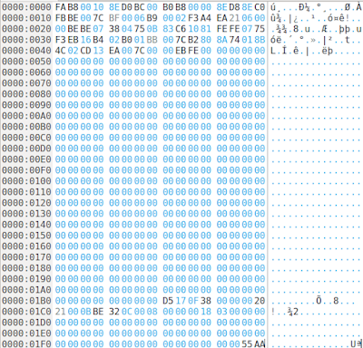
First sector of the image which is the MBR

(2) In order to find the files stored in this disk image, we need to first locate the FAT partition. To locate FAT partition we have to find it by reading the partition table inside MBR properly. By looking at the structure of the MBR, we can see that partition table takes 64 bytes long area at the end of the partition right before the last two bytes signature. To make our life easier, let's just copy partition table and paste into a new tab in Okteta.

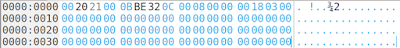
Partition table which is 64 bytes long

(3) Once again, a glance at the structure of a partition table entry tells us that an entry in the table is 16 bytes long and the whole table is 64 bytes long. That means it can accommodate up to 4 partition entries. Empty partition entries are filled with zeros. Now, when we look at the partition table that we just extracted from our image, we can see that there's only one partition entry there. Following is that entry.

        00202100 0BBE320C 00080000 00180300

(4) Let's start interpreting this partition entry. The very first byte in this entry tells us whether this partition is bootable or not. That means whether this partition contains an operating system or not. The first byte contains 0x00. That means, no this is not a bootable partition.

(5) Another useful information is what type of file system is available on this partition. That information is available in the offset 0x04 location in the partition entry. That value is 0x0B as you can see. Our reference document tells us that this value means, our partition is a FAT32 partition. Great! We know about FAT file system. So we will be able to explore this partition.

(6) Next question that arises is where is this FAT32 partition in the disk image? How to locate it? Again our reference document tells us that the offset 0x08 of the partition entry contains 4 bytes which specify the starting sector of this partition. When you look at the partition entry, you can see that this value is 00 08 00 00. So, this value represents the starting sector of the FAT32 partition. We need to interpret this number carefully. This is a number stored in little-endian format. That means, the last byte is the most significant byte. We have to reverse the order of these bytes before interpreting.

    The number you get once you revert it from little-endian format is 00 00 08 00. Let's use the calculator to convert this hexadecimal number to decimal. The decimal value is 2048. That means This FAT32 partition begins at the sector number 2048. Let's go there and see this partition.

    But, wait! Our hex editor shows offsets in bytes, not in sector numbers. So, we need to find the byte offset of this sector number 2048. We can easily do that by multiplying 2048 by 512 because there are 512 bytes in a sector.

    2048 x 512 = 1048576

    Again, we have to convert this decimal byte offset 1048576 into hexadecimal before going there. Ask help from the calculator for that too.

    1048576 (decimal) = 100000 (hexadecimal)

    Now, 100000 is the byte offset in hexadecimal where you can find the FAT32 partition.

(7) Instead of scrolling down to find the above offset, we have an easy way in Okteta editor. You can go to Edit menu and select Go to Offset... option. Then, at the bottom of the Okteta window, you get a text field where you can specify where you want to go. Put 100000 there and hit Enter.

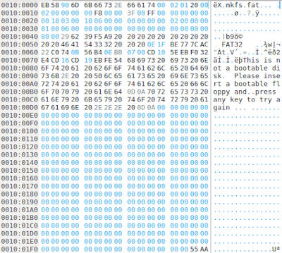
First sector of the FAT partition which is the boot sector.

Now, we are at the FAT32 partition. It's time to take the reference document which has FAT32 related data structures to your hand. We need it from here onwards.

(8) The very first sector in the FAT32 partition is called boot sector. There are lots of useful information in this sector. Let's go through some of the important ones. It is a good idea to copy the first 48 bytes into a new tab in Okteta for our convenience. The information we are looking for are in this area.

First 48 bytes of the boot sector in a new Okteta tab.

(9) In this boot sector, offset 0x0B contains 2 bytes which specify the number of bytes per sector. The value you can find in this location is 00 02 and as usual this is in little-endian. Convert it back to big-endian and you get 02 00. Converting this hexadecimal number to decimal gives us 512. That means, clearly 512 bytes per sector rule applies within this FAT32 partition.

(10) In this boot sector, offset 0x0D contains a byte which specify the number of sectors per each cluster. Let's see what is in that location. In our boot sector, this location contains the value 0x01. Converting from hexa to decimal give us 1 as the answer. That means, each cluster in this partition is actually a single sector. Simple enough.

(11) In this boot sector, offset 0x0E contains 2 bytes which specify the number of reserved sectors in this FAT32 partition. That means, the number of sectors between the beginning of the partition and the FAT1 table. The value in that offset gives us 20 00 which is in little-endian. In big-endian, we get the hexadecimal value 0x0020 which is 32 in decimal. That means, there are 32 sectors in the reserved area before the FAT1 table. It is important to note that these 32 sectors include the boot sector itself. In other words, boot sector is just another sector in the reserved area.

(12) In this boot sector, offset 0x10 contains a byte which specify the number of FAT tables we have in this partition. Usually there are 2 tables called FAT1 and FAT2, but it's better to see whether it's true. The value in that offset specify the value 02 in hexadecimal. In decimal, the value is 2 and that means we have two FAT tables indeed.

(13) In this boot sector, offset 0x11 contains 2 bytes which specify the maximum number of file entries available in the root directory. However that applies only to FAT12 and FAT16 versions of FAT. This partition that we are exploring is a FAT32 parition and in FAT32, the number of entries in the root directory is not specified here. So, we don't have to interpret anything here.

(14) The offset 0x16 in the boot sector has 2 bytes which specify the number of sectors in each FAT table. There's an important thing to note here. If these two bytes contain some non-zero value, we can take that number. However, if the location contains all zeros in those two bytes, that means, the space is not enough to specify the information. In that case, we have to go to the offset 0x24 and interpret 4 bytes there.

    The value in the two bytes at offset 0x16 gives us 00 00 in our image. That means we have to go to 0x24 and take the 4 bytes it has. In our image, we have 18 06 00 00. Converting from little-endian gives us the value 00 00 06 18 which is 1560 in decimal. Therefore, we conclude that there are 1560 sectors in a FAT table. Since we have two FAT tables, they take up twice of that space.

(15) In this boot sector, offset 0x2C contains a byte which specify the first cluster of the root directory. This information is useful when we later recover file data. The value in that location is 0x02 which is 2 in decimal. That means, there are two clusters in this disk image before the root directory, namely cluster 0 and cluster 1. You will see how this information becomes useful later.

(16) Now, we have enough information to locate the root directory of this FAT32 partition. Here's how we calculate the location. The root directory is located right after the two FAT tables. That means, we just have to walk through the reserved area from the beginning of the partition, then through the FAT1 and FAT2 tables and there we find the root directory.
 

Offset to root directory = (number of sectors in reserved area) + (number of sectors in a FAT table) x 2
                                 = 32 + (1560)x2
                                 = 3152 sectors.
                                 = 3152 x 512 bytes
                                 = 1613824 bytes
                                 = 0x18A000 bytes (in hex)

        There's a tricky thing here. This offset specifies the location from the beginning of the partition. Unfortunately, we are dealing with an entire disk image. The FAT32 partition starts at 0x100000 bytes location as we found previously by looking at the MBR. Therefore,
 

Offset to the root directory (in our disk image) = 0x100000 + 0x18A000 = 0x28A000 bytes.

Let's jump to this offset in Okteta and see what we find there.

Root directory of the FAT partition in a new Okteta tab.

Yup, this location indeed looks like the root directory.

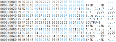
(17) Root directory contains entries which are 32 bytes long. At first glance, you can see that there are 6 entries in this root directory. For our convenience, let's copy the whole root directory to a new tab in Okteta.

(18) Now our reference document tells are which bytes in a directory entry specifies which information. The first byte of a root directory entry is important. If a file is deleted, the first byte is simply set to 0xE5. Now you can identify 3 entries which has the first byte set to 0xE5 and therefore simply deleted files. I'm going to pick just one file from this root directory and explore it. It's up to you to deal with remaining files.

(19) I'm selecting the entry at the offset 0x000000A0 to deal with. It's the last entry in our root directory. According to our reference document, first 11 bytes of a directory entry contains file name. A dot (.) is implied between the two bytes at locations 0x07 and 0x08. The values in those 11 bytes in our directory entry are as follows.

        4E 4F 54 45 53 20 20 20 54 58 54

We simply have to convert each byte into the relevant ASCII character using an ASCII code chart.

        NOTES.TXT

(20) In this root directory entry, the offset 0x0E contains 2 bytes which represent the file creation time.  The value in that location is 95 A4 in little-endian. We convert it to big-endian to get A4 95 which is 1010010010010101 in binary. From this number, first 5 bits represent the hour. Next 6 bits  represent the minute and the last 5 bits represent the seconds divided by 2.

    Hour: 10100 = 20
    Minute: 100100 = 36
    Second: 10101 = 21 -> 21x2 = 42

    Therefore, creation time = 20:36:42

(21) In this root directory entry, the offset 0x10 contains 2 bytes which represent the file creation date.  The value in that location is 66 4B in little-endian. We convert it to big-endian to get 4B 66 which is 0100101101100110 in binary. From this number, first 7 bits represent the year since 1980. Next 4 bits  represent the month and the last 5 bits represent the day of the month.

    Year: 0100101 =  37 -> 1980+37 = 2017
    Month: 1011 = 11
    Day: 6

    Therefore, creation date: 2017/11/06

(22) In this root directory entry, the offset 0x12 contains 2 bytes which represent the file accessed date. The value in that location is 66 4B in little-endian. That is same as the file creation date which we calculated previously. So, the accessed date is same as the created date for this file.

(23) In this root directory entry, the offset 0x16 contains 2 bytes which represent the file modified time. The value in that location is 95 A4 in little-endian. That value is similar to the file creation time. so, no need to calculate it again in this case.

(24) In this root directory entry, the offset 0x18 contains 2 bytes which represent the file modified date. The value in that location is 66 4B in little-endian. That value is similar to the file creation date. so, no need to calculate it again in this case.

(25) Now we are ready to process the the contents of the file. The location of the first cluster that belongs to this file contents is given in two fields of the root directory entry.  The offset 0x14 gives the high-order 2 bytes. The offset 0x1A gives the low-order 2 bytes. Remeber that each value is in little-endian.

    High order value: 00 00 -> little-endian to big-endian -> 00 00
    Low-order value: 08 00 -> little-endian to big-endian -> 00 08

    Cluster number = 00 00 00 08 = 8 (decimal)

    Therefore, the first cluster where our file contents can be found is cluster 8.

    Calculating the byte offset to the cluster number 8 is again bit tricky. This is how we handle it. In the point (15), we found that there are 2 clusters before the root directory.  That means from the root directory to the file data location, there are 6 clusters because 8-2 = 6. Therefore, we can calculate to the byte offset to this file location  from the root directory as follows. We simply multiply 6 clusters by the number of sectors per cluster (which is 1) and by number of bytes per sector (which is 512).
 

byte offset from the root directory to the file data = 6 x 1 x 512 = 3072 (decimal) = 0xC00

    Now, if we add this offset to the offset of the root directory from the beginning of the disk image, we get the location of the file data exactly from the beginning of the disk image.

    absolute offset to the file data =  (byte offset to the root directory) + 0xC00
                                             =  0x28A000 + 0xC00
                                              = 0x28AC00

Now, let's goto this offset and you will see the file contents.

That's all folks!

~*************~

Creating a Raw Image File, Partition and Format It

When playing with file system related stuff, especially for studying how they work at the low level with a hex editor, we are in need of many disk images. In such situations, instead of acquiring real disk images, it is possible to artificially create disk images on demand with any number of partitions we want with different file system times with a custom size. In this blog post, I'm writing down the steps to follow, in order to create such a disk image with the partition table and a single FAT32 partition.

(1) Creating a 100MB raw file.

    dd if=/dev/zero of=image.dd iflag=fullblock bs=1M count=100 && sync

(2) Mounting the blank image into a loop device.

    sudo losetup loop0 image.dd

Now, if you run the command losetup, you should see an output where loop device loop0 is mounted with the image.

(3) Let's partition this new loop device using GParted tool. For that, first we should install it.

    sudo apt-get install gparted

(4) Open the GParted tool using the following command. Follow the steps of the screenshots in order to create the partition table and a FAT32 partition.

    sudo -H gparted /dev/loop0

 

GParted window.

Creating a partition using the "Device" menu.

Select partition type "msdos" and apply.

Our drive with a partition table but no partitions yet.

Creating a partition using the "Partition" menu.

Select "File system" type as fat32 and click add.

Newly created partition. Size is smaller because of the partition table, etc.

Click on the button to apply file system creation operation to the drive.

Click apply to go ahead.

All done. Click "close" to finish and close the GParted window.

(5) Unmount the loop device.

    sudo losetup -d /dev/loop0

Now, our image.dd file contains a partition table of msdos type and a single partition with FAT32 file system. We can check it using a command available on Sleuthkit as follows.
 

  sudo apt-get install sleuthkit
  mmls image.dd

 

Cheers!


References:
[1] https://askubuntu.com/questions/667291/create-blank-disk-image-for-file-storage

~************~

3. Notes on Machine Learning: Basics of Neural Networks

Neural Networks is an interesting branch in machine learning which attempts to mimic the functionality of neurons in human brain. A neural network consists of the input feature vector \(X\) to a node, the hypothesis function which is sometimes called the activation function running inside a node and finally the output of the function. Instead of having a single activation unit, we can have multiple layers of activation nodes. The input vector layer is considered as the first layer while there are multiple hidden layers (layer 2, layer 3, etc) before the output layer.

The \(\theta\) parameter set is not a single vector like in linear regression and logistic regression in this case. This time, in neural networks, we have a  \(\theta\) parameter set between every two layers. For example in the above figure, we have three layers, and therefore, we have two \(\theta\) sets. The arrows going from layer 1 to layer 2 represent the parameter set \(\theta^{(1)}\). The arrows going from layer 2 to layer 3 represent the parameter set \(\theta^{(2)}\). The upperscript number within the brackets represent the origin layer this parameter set belongs to. Furthermore, \(\theta^{(1)}\) is a matrix with 3x4 dimentions. There, every raw represents the set of arriows coming from the layer 1 features to a node in layer 2. For example, the element \(\theta^{(1)}_{10}\) represents the arrow to \(a_1^{(2)}\) from \(x_0\). The element \(\theta^{(1)}_{20}\) represents the arrow to \(a_2^{(2)}\) from \(x_0\).

$$\theta^{(1)} = \begin{bmatrix}\theta^{(1)}_{10} & \theta^{(1)}_{11} & \theta^{(1)}_{12} & \theta^{(1)}_{13}\\\theta^{(1)}_{20} & \theta^{(1)}_{21} & \theta^{(1)}_{22} & \theta^{(1)}_{23}\\\theta^{(1)}_{30} & \theta^{(1)}_{31} & \theta^{(1)}_{32} & \theta^{(1)}_{33}\end{bmatrix}$$

Meanwhile \(\theta^{(2)}\) is a raw vetor (1x4) in this case. This is because there are 4 arrows coming from the layer 2 nodes to the layer 1 node.

$$\theta^{(2)} = \begin{bmatrix}\theta^{(2)}_{10} & \theta^{(2)}_{11} & \theta^{(2)}_{12} & \theta^{(2)}_{13}\end{bmatrix}$$


The hypothesis function in thse neural networks is a logistic function just like in the logistic regression.
 $$h_\theta (x) = \frac{1}{1 + e^{- \theta^T x}}$$
For a neural network like the one shown in the above figure, we can calculate the activation and get the final output inthe following way. There, \(a_1^{(2)}\) represent the activation node 1 in the layer 2 (hidden layer). Similarly \(a_2^{(2)}\) represent the activation node 2 in the layer 2 and so on.

$$a_1^{(2)} = g(\theta_{10}^{(1)} x_{0} + \theta_{11}^{(1)} x_{1} + \theta_{12}^{(1)} x_{2} + \theta_{13}^{(1)} x_{3})$$

$$a_2^{(2)} = g(\theta_{20}^{(1)} x_{0} + \theta_{21}^{(1)} x_{1} + \theta_{22}^{(1)} x_{2} + \theta_{23}^{(1)} x_{3})$$

$$a_3^{(2)} = g(\theta_{30}^{(1)} x_{0} + \theta_{31}^{(1)} x_{1} + \theta_{32}^{(1)} x_{2} + \theta_{33}^{(1)} x_{3})$$

$$h_\theta (x) = a_1^{(3)} = g(\theta_{10}^{(2)} a_{0}^{(2)} + \theta_{11}^{(2)} a_{1}^{(2)} + \theta_{12}^{(2)} a_{2}^{(2)} + \theta_{13}^{(2)} a_{3}^{(2)})$$
Since the hypothesis function is a logistic function, the final output we get is a value between 0 and 1. What we do to have a multiclass classifier is, having multiple nodes in the output layer. Then, we get a unique output value from each node in the output layer representing a specific class.

~************~

2. Notes on Machine Learning: Logistic Regression

Unlike regression problems where our objective is to predect a scalar value for a given set of values in features, in classification problems our objective is to decide a discrete value from a limited set of choices. Therefore, we are not going to use Linear Regression in classification problems. Based on how many categories we have to classify our input, we have two types of problems; binary classification and multiclass classification.

In binary classification problems, there are only two possible outputs for the classifier; 0 or 1. Then as it is obvious, multi-class classification problems can have multiple output values such as 0, 1, 2, .. however there's a descete set of values, not infinite. When solving these classification problems, we develop machine learning models which can solve binary classification problems. When we have multiple classes in a problem, we use multiple binary classification models to check for each class.

Logistic Regression:

In order to maintain the prediction output between 0 and 1, we are using a zigmoid/logistic function as the hypothesis function. Therefore, we call this technique, Logistic Regression. Hypothesis function of the logistic regression is as follows.
$$h_\theta (x)=\frac{1}{1+e^{-\theta^T x}}$$
The vectorized representation of this hypothesis would look like the following.
$$h=g(X\theta)$$
For any input value in \(x\), this logistic regression hypothesis function outputs a value between 0 and 1. If the value is closer to 1, we can consider it as a classification to the class 1. Similarly, if the value is closer to 0, we can consider the classification as 0. On the other hand, we can consider the output value between 0 and 1 as a percentage probability to classify as the class 1. For example, if we receive the output 0.6, it means there's a \(60\%\) probability for the input data to be classified to class 1. Similarly, if we receive the output as 0.3, it means there's a \(30\%\) probability for the input data to be classified to class 1.

Cost Function:

The cost function of the logistic regression is different from the cost function of the linear regression. This cost function is designed in a way where if the logistic regression model makes a prediction with a \(100\%\) accuracy, it generates a zero cost penalty while if it maks aprediction with a \(0\%\) accuracy, it generates an infinite penalty value.
$$J(\theta)=-\frac{1}{m}\sum_{i=1}^{m} [y^i log(h_\theta(x^i)) + (1-y^i) log(1-h_\theta(x^i))]$$
A vectorized implementation of the cost function would look like the following.
$$J(\theta)=\frac{1}{m}(-y^Tlog(h) - (1-y^T)log(1-h))$$

Gradient Decent:

In order to adjust the parameter vector \(\theta\) untill it fits properly to the training data set, we need to perform gradient decent algorithm. Following line has to be repeated for each \(j\) simultaneuously which represent the parameters \(\theta\). In this gradient decent algorithm, \(\alpha\) is the learning rate.
$$\theta_j=\theta_j - \frac{\alpha}{m}\sum_{i=1}^{m}(h_\theta(x^i) - y^i)x_j^i$$
A vectorized implementation of the gradient decent algorithm would look like the following.
$$\theta = \theta - \frac{\alpha}{m}X^T(g(X\theta) - y)$$

Multiclass Classification:

The above technique works for classifying data into two classes. When we encounter a multiclass classification problem, we should train a logistic regression model for each class. For example, if there are 3 classes, we need three logistic regression models trained to distinguish between the targetted class and the others. In this way, we can solve  multiclass classification problems using logistic regression.

Overfitting and Underfitting:

Overfitting and Underfitting are two problems which can occur in both Linear Regression and Logistic Regression algorithms. The former problem occurs when our model fits too accurately to the training data set so that in does not represent the general case properly. The latter issue occurs when our model does not even properly fit to the training data set.

Regularization is a nice technique to solve the problem of overfitting. What happens there is we maintain the values of \(\theta\) parameter vector in a smaller range in order to stop the learning model curve from adjusting too agressively. This is achieved by adding extra weights to the cost function. It prevents the medel from overfitting to the training dataset. We can use this technique in both linear regression and logistic regression.

Regularized Linear Regression:

The gradient decent algorithm for the linear regression after adding regularization looks like the following. The two steps has to be repeated in each step of the gradient decent. There, \(j\) stands for 1, 2, 3, .. which represent each \(\theta\) parameter in the hypothesis. \(\lambda\) is the regularization parameter.
$$\theta_0 = \theta_0 - \alpha \frac{1}{m} \sum_{i=1}^{m}(h_\theta(x^i) - y^i) x_0^i$$
$$\theta_j = \theta_j - \alpha [(\frac{1}{m} \sum_{i=1}^{m}(h_\theta(x^i) - y^i) x_j^i) + \frac{\lambda}{m} \theta_j]$$

Regularized Logistic Regression:

The gradient decent algorithm for the logistic regression after adding regularization looks like the following.
$$\theta_0 = \theta_0 - \alpha \frac{1}{m} \sum_{i=1}^{m}(h_\theta(x^i) - y^i) x_0^i$$
$$\theta_j = \theta_j - \alpha [(\frac{1}{m} \sum_{i=1}^{m}(h_\theta(x^i) - y^i) x_j^i) + \frac{\lambda}{m} \theta_j]$$
Of course, it looks like the regularized linear regression. However, it is important to remember that in this case, the hypotheis function \(h_\theta (x)\) is a logistic function unlike in the linear regression.

~**********~ 

Ireland's Space Week in 2017

Image credit: @Lana_Salmon

Last week in Ireland is called Space Week where the focus was on promoting space exploration and related science and technologies among people. This time for Ireland is so special because they are building a cube satellite with the joint contribution of universities and Irish space technology companies. During this space week, there were so many events organized by different institutions all over the Ireland. Even though I was busy with my work, somehow I finally managed to attend to an interesting event organized by the University College Dublin.

The event was titled Designing for Extreme Human Performance in Space which was conducted by two very interesting personalities. The first person was Dava J. Newman, who is a former deputy administrator of NASA and currently works for the MIT. The second person was Guillermo Trotti, who is a professional architect and has worked for NASA on interesting projects. Seeing the profiles of these two speakers attracted me to attend to the event. The session was held for about an hour and a half where the two speakers shared the time to talk on two different areas they are interested in. Finally, the session was concluded with a Q&A session.

Image credit: @ASayakkara

In her presenation, Dava talked about the extreme conditions in space which raise the requirement of designing life support systems to assist astronauts. When she asked from the famous astronaut Scott Kelly (@StationCDRKelly), who spent a year in ISS, about what would be the most needed thing if we are to improve in space technology, he has responded that life support systems to ease the operation of astronauts on space is the most needed thing. Dana presented the work she is involved in designing a new kind of space suit for astronauts to use on other planets such as Mars. The pictures she showed indicates a skin-tight suit which is custom designed to the body specification of an astronaut very much like a suit from a sci-fi movie.

Gui Trotti in his presentation talked specifically about his architectural interest on building habitable structures for humans on the Moon and Mars. As a professional architect, he is so inspired to bring his skills into human colonies in outer space. During that presentation, his mentioned three things that inspired me so much. The first is the fact that when an astronaut goes to space and turn back to look at his home planet, all the borders and nationalistic pride goes away and comes the feeling of we all are one human race and that planet Earth is the only home we have. Secondly, he described his tour around the world in a sailing boat which reminded him that space exploration is another form of human courage to explore and see the world. Finally, he said that his dream is to build a university on the moon one day to enable students from the Earth to visit and do research appreciating our home planet.

During the Q&A session, a lot of people asked interesting questions. Among those, one question was about the commercialization of space. They responded with the important fact that there is a potential of performing commercial activities such as manufacturing on space, especially the things which can be done easily on zero gravity environments rather than on the surface of the Earth. Various things such as growing food plants and 3D printing have been tried on the ISS towards this direction. In the near future such as a decade along the line, we would be able to see much more activities from the private sector on space than today. They are so positive about the progress in this area.

Even though I'm not working in anywhere related to space exploration,  I'm always fascinated by this topic and I will continue to be.

~*********~

1. Notes on Machine Learning: Linear Regression

Machine Learning is a hot topic these days since various kinds of applications rely on Machine Learning algorithms to get things done. While learning this topic, I will be writing my own notes about it as article serious in this blog for my own future reference. The contents might be highly abstract as this is not a tutorial aimed at somebody to learn Machine Learning by reading these notes.

Definition:

According to the definition of Tom Mitchell, Machine Learning is defined as  "A computer program is said to learn from experience E with respect to some class of tasks T and performance measure P if its performance at tasks in T, as measured by P, improves with experience E." Basically, we are enabling computers to do things without explicitly programming them to do it.

Categories of Machine Learning:

There are two broad categories of Machine Learning algorithms. The first is Supervised Learning and the second is Unsupervised Learning. There are various sub categorizations under these categories which can be illustrated as follows.

Machine Learning Models:

A model is a function (ie. hypothesis) \( h(x) \) which provides the output value \( y \) for a given input values \( x \), based on previously given leaning dataset \( X \) and output set \( Y \). The input values \( x \) are called features. A hypothesis function in Linear Regression with one feature would look like the following.
$$ h(x) = \theta_{0} x_{0} + \theta_{1} x_{1} $$

The first feature \( x_{0} \) is always set to 1 while the second feature \( x_{1} \) is actually the feature used in this model. The parameters \( \theta_{0} \) and \( \theta_{1} \) are the weight of the features to the final output and therefore, they are the values we are looking for in order to build the linear regression model for a specific dataset. The reason why we have an extra feature in the beginning which is always set to 1 is that it is easy to perform vecterized calculations (using matrices based tools) when we have it in that way.

Cost Function:

In order to measure the accuracy of a particular hypothesis function, we use another function called cost function. It is actually, a squared mean error function between the difference of predicted output value and the true output value of the hypothesis. By adjusting the values of the parameters \( \theta_{0} \) and \( \theta_{1} \) in the hypothesis, we can minimize the cost function and make the hypothesis more precise.
$$J(\theta_{0},\theta_{1}) = \frac{1}{2m} \sum_{i=0}^{m} (h_\theta(x_i) - y_i)^{2}$$

Gradient Descent:

In this algorithm, what we are doing is keep adjusting the parameters \( \theta_{0} \) and \( \theta_{1} \) until the Cost Function evetually becomes the minimum it can get. That means, we found the most accurate Model for the training dataset distribution. So, in order to adjust the parameters \( \theta_{0} \) and \( \theta_{1} \), we perform the following step over and over again for \( \theta_{0} \) and \( \theta_{1} \). In this equation, \( j \) is 0 and 1 in two steps.
$$\theta_{j} = \theta_{j} - \alpha \frac{\partial }{\partial \theta_{j}} J(\theta_{0},\theta_{1})$$

~*********~

Upgrading Octave to the Latest Version on Ubuntu

These days, I'm following the machine learning course in Coursera conducted by Andrew Ng. In this course, the most important thing is the exercises. Since I'm on Linux platform with an Ubuntu 16.04 version, I installed Octave for this work as follows.

sudo apt-get update

sudo apt-get install octave

The latest Octave version on Ubuntu 16.04 repositories is 4.0.0. However, while working on the exercise of this course, I realized that this version has some problems which make it unsuitable to use with the sample Octave scripts provided in the course. The advice was to use a higher version of Octave than 4. In order to do that, we have to add a new PPA to the system as follows.

sudo add-apt-repository ppa:octave/stable
sudo apt-get update

Now, let's remove the whole previous Octave version and install from the beginning with the new PPA.

sudo apt-get remove octave

sudo apt-get autoremove

sudo apt-get update

sudo apt-get upgrade

sudo apt-get install octave

Now, the version we get is the latest version in the new PPA. You can check it by first starting Octave and typing "version" on the prompt. The version I got was Octave 4.2.1.

References:

[1] https://launchpad.net/~octave/+archive/ubuntu/stable

"AI and The Future" by Margaret Boden

Last Tuesday, I attended to an interesting guest talk by Professor Margaret Boden from University of Sussex under the topic AI and The Future. Even though I'm not much into Artificial Intelligence topic, I decided to attend to this session simply driven by curiosity. Most importantly, this is the first session of its kind I'm attending in UCD and therefore I just wanted to see how guest talks are going to be here. The talk was delivered at the Moore Auditorium in UCD Science Center.

In her talk, she mostly talked about the implications of AI systems in our everyday life and what she believes as the things to be worried about. The concern she pointed out in her talk is that, when AI systems replace human presence from certain activities, we tend to receive bad results and bad long term impacts on our society even though AI application can seem to be useful and makes life easier. In order to support her point, she took a broad range of examples including autonomous drones, AI systems to take care of elderly and kids.

Even though I have a habit of posing a question when I attend to sessions like these, unfortunately, I couldn't ask a question in this session. They were running out of time and many people wanted to ask questions. However, I feel that it's worth the time I invested on attending this guest talk. I will hopefully attend to the future sessions organized by them.

Demodulating AM Signals using GNURadio

I have been using GNURadio for different purposes for some time. However, in most of those times, I used either a very simple flow graph created by myself or a complicated flow graph created by somebody else. Therefore, in the case of complicated flow graphs, I didn't even bother to explain how they work as I didn't really understand their internal functionality. Yesterday, I came across a need to demodulate a signal captured from an RTL-SDR and saved to a file. From the output I observed through the GQRX tool, the signal is modulated using Amplitude Modulation (AM). I wanted to implement a demodulator by myself and therefore I searched the web for a tutorial regarding this kind of stuff. I found a tutorial given in the references section which was really useful [1].

In the rest of this post, I will be explaining how this AM demodulation flow graph is implemented and the functionality of each block according to my understanding. There can be missing details and inaccurate things. If you notice some glitch, please be kind to let me know by leaving a comment. Here we go.

(1) The signal I'm trying to demodulate is in 32MHz frequency and therefore, I tuned an RTL-SDR dongle to that frequency and captured data to a file with a sample rate of 1.8MHz. The tool I used for this purpose is a command line tool called osmocom_fft which comes in handy when we need to save captured data into the .cfile format.

(2) Let's start with a File Source block in the flow graph. Double click on it and then browse to select the source file which contains data. Set the Repeat option to yes.

(3) The data in the file is recorded in 1.8MHz sample rate and the samples are centered to the 32MHz signal. If we draw an FFT spectrogram from the raw data of the file, we will see the X-axis from (32-1.8)MHz to (32+1.8)MHz. However, the real AM signal does not span such a width. The real signal was within about 5kHz width (not exactly). Therefore, let's narrow down our data scope to somewhere about 10kHz in order to focus on our signal. To narrow down our spectrum information from 1.8MHz width to 10kHz, we need to resample the data. So, let's use a Rational Resampler block as the next step.

In the Rational Resampler block, we have two important parameters; Interpolation and Decimation. Interpolation value represents the number by which the input signal's sample rate is multiplied. Decimation value represents the number of which the input signal's sample rate is divided. In order to resample a 1.8MHz signal into the 1kHz signal, we have to divide the input by 180 and multiply by 1. That means, set the Interpolation to 1 and Decimation to 180 in the Rational Resampler block.

Here, instead of directly putting the resampling value 18 in the field, let's make the value a variable so that later we can change it easily. Therefore, add a variable called resamp_factor and set the value to 180.

(4) It is important to note that the purpose of the Rational Resampler is to change the sampling rate of some data. The output of the current setup is a signal with a sample rate of 10kHz. However, to actually isolate the signal we need to extract, we should filter out the other frequencies and keep the target frequency. This is where we need a filter. The target signal is about 5kHz wide. And it is centered at the 35MHz. Therefore we need to add a Low Pass Filter block with a cutoff frequency at 5kHz. Any signals which contain more than 5kHz components will be removed by this block.

When setting the sample rate of the Low Pass Filter block, it is important to set it to the value (samp_rate / resamp_factor) since, the sample rate is now changed by the previous block, the Rational Resampler.

(5) Now we are focused to the exact signal we need to demodulate. Since we are interested in amplitude modulation (AM), we are interested in the amplitude of the signal. We can convert the complex data we were receiving out of the filter to a series of numbers which represent the amplitudes using a Complex to Mag module. Now the output of this module is basically the demodulated base band signal.

(6) It is useful to have a way to increase and decrease the amplitude of the demodulated signal in order to listen to it conveniently. In order to achieve that, we add a Multiply Const block. In the constant field, instead of adding an exact number, we put a name called volume. Then, we should add WX GUI Slider block separately. Set the ID of this new block to be volume. Set the minimum value 0 and maximum value 10 with a number of steps set to 100. Now, when we change the volume in the WX GUI slider, it will change the value in the Multiply Cont block.

(7) Before we add an audio sink to listen to the sounds, we need one more thing. Since an audio sink would need the sample rate to be around 48kHz, let's resample the sample rate of the current setup from 10kHz to 48kHz by using another Rational Resampler. Set the decimation to 10 and interpolation to 48 for the obvious reasons.

(8) Now the last thing. Add an Audio Sink block and set the sample rate to 48kHz. If you think it's useful, add a WX GUI Scope Sink which will show the waveform of the audio signal being heard. The sample rate of that block too has to be 48kHz.

Run this flow graph and listen to the output sound. You should be able to hear the demodulated signal. In case you need to take a look at the original GNURadio Companion based file I created for the above AM demodulator, download the GRC file in the GIST given in this link.  Cheers!

References: 

[1] https://www.csun.edu/~skatz/katzpage/sdr_project/sdr/grc_tutorial3.pdf

~*******~

Memories of Staff Development Program at University of Kelaniya

While being a lecturer in University of Colombo School of Computing, I had a requirement of following a staff development program as one of the conditions to get confirmed in my position. Even though I have expertized in my own field of study, there's no doubt that I'm not a complete person as a lecturer. How to properly involve in the teaching and learning process as a lecturer is something I have to learn separately. The university grants commission (UGC) of Sri Lanka has accredited several staff development programs (SDC) offered in different universities in Sri Lanka. Among these, I selected the SDC program in University of Kelaniya for me.

Since, I did my bachelors degree in University of Colombo and joined the staff of the same university, I had never got a chance to participate to a course in another university in Sri Lanka as a student. I have been to University of Sri Jayawardanepura, but as a visiting lecturer, not as a student. Therefore, me joining the SDC program in University of Kelaniya is the first time I played the student role in another university. Prof. Dilkushi Wettewe who was the director of the SDC program then, assisted me so much when I contacted her to get further details. Even though University of Kelaniya is located a little bit far away from University of Colombo, I considered it has a positive change to visit a new place and be a student. It indeed became a whole new experience.

The course was scheduled to be in every Friday and the course goes from the morning to the evening across the whole day. The participants to the course included new lecturers from various universities in Sri Lanka such as University of Kelaniya, University of Vocational Technology and Bhikkhu University Anuradhapura. I was the only participant from University of Colombo. Before attending to the course, I never realized that I have so much to learn about teaching and learning process as a lecturer. The course starts with the introduction to the university system in Sri Lanka and how the parliamentary acts have formally established the universities in Sri Lanka. Throughout the course, we studied various aspects of university education. The most exciting thing I came across by attending to the SDC program is the participants I got to know there. I believe that the contacts I made with the people will remain for the rest of my carrier.

At the last day of the course, we had a little ceremony to award the certificates to the attendees of the course where I performed the vote of thanks. I was lucky to receive a best portfolio award which was awarded only to 5 participants of the course. I'm really happy about the opportunity I got to take part in the program.

~************~

Inspectrum: A tool to inspect signals from SDR

If we are using a software defined radio (SDR) device to capture some signals and planning to analyze it later, we might need a good software to visualize the data. The most obvious solution is to use GNURadio Companion itself as it has the required modules to plot waveform, FFT and waterfall graphs. However, today I found another useful tool which we can use to visualize and inspect recorded signals. It is called Inspectrum. Following are the steps to easily install it and try using a dummy data file generated using GnuRadio Companion.

sudo apt-get update
sudo apt-get install inspectrum
sudo apt-get install gnuradio

Now, let's start GnuRadio Companion by using the following command on the terminal.

gnuradio-companion

Create the flow graph shown in the following figure. It reads from a sample Wav file we have stored in our computer and writes it to a new file in the correct format which we need. The file extension of the file we write to should be .cfile in order for the Inspectrum tool to recognize it properly. Let's say our output file name is mydata.cfile.

Flow graph to generate sample data

It's time to try the new tool we wanted to see. Run the following command in the terminal to start Inspectrum with the data file we created.

inspectrum mydata.cfile

Inspectrum window with sample data file

Writing in Sinhala (සිංහල) using Latex (a follow up post)

Sometime back, I wrote a blog post about preparing Latex documents with Sinhala language [1]. I received very good feedbacks for that post and encouraged me to explore more. However recently, I came across a question posted in Stack Exchange regarding Latex documents in Sinhala [2]. The nice thing was that my original blog post was mentioned in that thread. I jumped in and tried to help the person who raised the question. This attempt helped myself to understand another important thing which is about how to use any Sinhala font we want in our Latex documents.

In this article, I decided to write down those simple steps of getting a Sinhala Latex document with our favorite Sinhala font for my future reference. Here we go.

(1) First of all, we need Latex with all the packages installed in our computer. I'm using a 64-bit Ubuntu 16.04 LTS machine. I can use the following command on the terminal to install Latex with all the packages.

sudo apt-get install textlive-full

(2) Now, open your favorite text editor and create a file with the name my-example.tex and save it in some directory (folder). This is the file where we will put our text contents.

(3) Now, you need to put the Sinhala font file in the directory. I'm going to use the fond called Iskoola Potha. It comes as a file with the file extension ttf. If you want the same file I used, you can download it from here [5]. I renamed the font file name to be iskoola-pota.ttf.

(4) Now, everything is set for us to write our Sinhala contents in the Latex file. Open the my-example.tex file and put the following content there.

1 2 3 4 5 6 7 8 9 10 11 12 13 14 15 16 17 18 19 20 21 22 23 24

\documentclass[12pt]{article} \usepackage[a4paper,left=2.5cm, right=2.5cm, top=2.5cm, bottom=2.5cm]{geometry} \usepackage{fontspec,xltxtra,xunicode} \setmainfont[Extension=.ttf, Language=Sinhala, BoldFont=iskoola-pota, ItalicFont=iskoola-pota]{iskoola-pota} \title{මාතෘකාව මෙතන ලියන්න} \author{අසංක සායක්කාර} \date{2017-07-16} \begin{document} \maketitle \section{සිංහල} මේ මම සිංහලෙන් සකස් කල ලිපියක්. මෙය සකස් කිරිඉමට මම \bf{ලේටෙක්} මෘදුකාංගය පාවිච්චි කලා. එය ඉතාම ප්‍රයෝජනවත් මෙවලමක් මට. \section{English} Some English here and there. \end{document}

(5) It's time to generate the PDF file and see how it looks like. Run the following command from the terminal for that.

xelatex my-example.tex

Now, you may notice that there's a PDF file generated in the local directory where you had your Latex and TTF files. Open the PDF file to see your output.

References:

[1] http://recolog.blogspot.ie/2016/08/preparing-latex-documents-in-sinhala.html
[2] https://tex.stackexchange.com/questions/359933/typing-in-sinhala
[3] https://www.icta.lk/fonts/
[4] http://studentlanka.com/2012/03/03/download-sinhala-and-tamil-unicode-fonts-free/

[5] http://www.download.aluth.lk/2015/01/iskoola-pota-font-download.html

OpenSSL on Linux Terminal for Cryptography

OpenSSL is the most important library we will be using if we are to use some cryptographic functions on a Linux computer. There are hundreds of variations of cryptographic algorithms and related functions are available on Linux terminal with OpenSSL. In this post, I would like to note down few useful things we can do with OpenSSL library on Linux.

Base64 Encoding:

When dealing with various files and data types, sometimes it is useful to convert everything into text format. Base64 is an encoding technique which we can use to convert different data into text format and then decode from text format to the original format. Let's see how we can do it.

First of all, let's select an image file in jpg format. We are going to encode this image file in base64 format as follows.

cat old-house.jpg | openssl enc -base64 >> encoded-image.jpg

Now, it you try to open the encoded image file, you will see that you cannot open in as a usual image file. However, the nice thing is, you can open the encoded image file using a text editor because the content is printable characters now. Let's decode the encoded image file back to the original format.

cat encoded-image.jpg | openssl enc -base64 -d >> decoded-image.jpg

Data Encryption Standard (DES):

DES is a little bit older data encryption algorithm which we don't have to use nowadays. Anyway, with OpenSSL library, we can use DES as follows to encrypt data.

openssl enc -des -a -in plantext.txt -out ciphertext.des

Once encrypted, we can use the following command to decrypt the data back to the plain text.

openssl enc -des -d -a -in ciphertext.des -out plaintext.tex

Advanced Encryption Standard (AES):

AES is a better and stronger encryption algorithm compared to DES. We can encrypt a file using AES and then decrypt the file back to the plain text using the following two commands.

openssl aes-256-cbc -in plaintext.txt -out ciphertext.aes

openssl aes-256-cbc -d -in ciphertext.aes -out plaintext.txt

Rivest, Shamir, Adleman (RSA):

When we are browsing web on our computer or mobile phone through a secure channel, the encryption algorithm which helps us most importantly is RSA. It is an asymmetric key encryption algorithm where we have two keys called as Public key and Private key. Private key is what we always keep to ourselves while the Public key can be distributed among everybody.

First of all, we need to generate a key pair in order to use RSA. Let's generate the private key and public key using the following two commands.

openssl genrsa -out private_key.pem 1024

openssl rsa -in private_key.pem -out public_key.pem -outform PEM -pubout

If you check the local directory where you were when running the above commands, now you should be able to see that two new files are created as private_key.pem and public_key.pem which are our keys. Now, we can encrypt data using RSA. Let's say we are going to encrypt a text file so that only a friend can see it. Then, we have to use the friend's public key during the encryption as follows.

openssl rsautl -encrypt -inkey public_key.pem -pubin -in plaintext.txt -out ciphertext.txt

Now, when your friend decrypt the cipher text, he or she should use his/her private key as follows.

openssl rsautl -decrypt -inkey private_key.pem -in ciphertext.txt -out plaintext.txt

Digital Signature of a Message:

When sending an encrypted message to someone, sometimes we need to prove that we are the person who sent the message. Just because we use RSA encryption as above, we cannot prove that we sent it. In order to prove the senders identity, we can use digital signatures. A digital signature is nothing other than just a Hash value of the original message encrypted using the private key of the sender. Since the private key of someone is always with that perform, a digital signature can be produced only by the owner of the sender's private key. We can digitally sign as follows using the RSA private key.

openssl dgst -sha256 -sign private_key.pem -out signature.txt plaintext.txt

Now, at the recipients side, he or she can verify the senders signature by decrypting the signature file using the senders public key (which is available) and then recalculate the Hash value of the original message. Following command illustrates that functionality.

openssl dgst -sha256 -verify public_key.pem -signature signature.txt plaintext.txt

There are so many things we can do with the OpenSSL library. It is up to you to explore it further.

References:

Friday, September 22, 2017