Signals against Noise in GNURadio

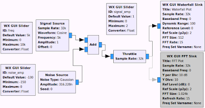
Figure - 1

In this article, I'm hoping to share a few more things I learned in GNURadio. To begin with, let's see what happens when a signal coming from a one source is mixed with another signal from another source. In particular, I'm adding a good signal with a noise generated from a noise source. Build the flow graph shown in figure-1 in GNURadio Companion (GRC) and it if needed, it's configuration file can be found here. You should notice that this time we are using three sliders, one to adjust the signal frequency, the second and third to adjust signal and noise amplitude. Our noise source is configured to generate some Gaussian noise in particular. We have plugged in a Waterfall sink and also an FFT sink. As you may have noticed in the flow graph, the FFT sink has become grey colored that means we have disabled that plot temporarily. We can enable and disable various blocks in the flow graph on the go. A block can be temporarily disconnected from the flow graph by right-click on the block and selecting 'disable' or 'enable' option. This option becomes handy where we need to try different parts of a flow graph without deleting the excess components which we may need later.

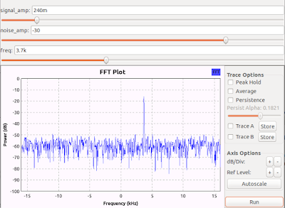Figure - 2

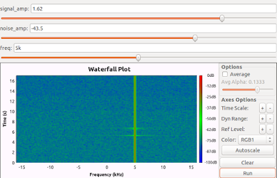Figure - 3

Running the flow graph with Waterfall sink and FFT sink separately results in plots shown in figure-2 and figure-3. Our three sliders will appear on top of the plots in each time. It is interesting to see how the increase of noise amplitude increases the noise floor making it's hard to find the signal. In figure-2, we can see a peak on top of the noise floor which is the signal. Similarly in figure-3, we can see a bright line which represent the signal. In this example, we had to enable and disable the two plots in order to view them separately. If we set them to display at the same time, sometimes the size of our screen may not be enough and most parts of the GUI windows will go out of the visible screen space. But, we have a solution for this which I explain in the next step.

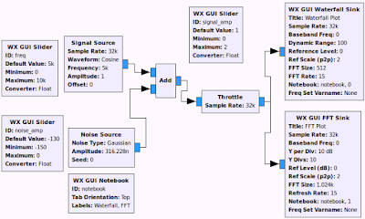Figure - 4

In order to easily view different GUI components such as FFT, Scope and Waterfall plots, we can arrange them into tabs in the window. For this purpose, first we should add a block called WX GUI Nootebook. Let's say we have to GUI plots currently in the flow graph which are a Waterfall Sink and an FFT sink. Double-click on the WX GUI Notebook block and in the 'Labels' field, add the content as ['Waterfall','FFT']. Set the ID field as Notebook. Now, double-click on the WX GUI Waterfall Sink block and in it's Notebook field, add the line notebook,0. Similarly, open the WX GUI FFT Sink block and in the Notebook field, add the line notebook,1. An example flow graph is shown in figure-4 and it's configuration file can be found here. Now, when we run the flow graph, we should be able to view the plots separately on different tabs as shown in figure-5. This is more convenient than displaying GUI components separately.

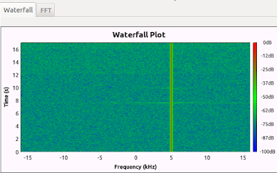Figure - 5

That's it!