Fundamentals of Radio Tomographic Imaging - Part 1

Nodes vs Links

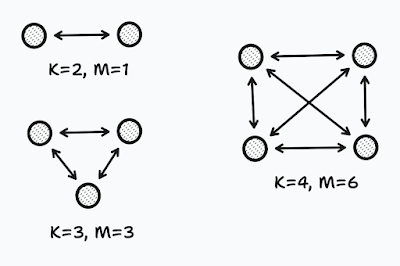
Consider a wireless network consisting of \(K\) number of devices. If each and every device is communicating with each other, there will be a wireless link between each and every pair of nodes. The number of such unique two-way links is depicted as \(M\). The following equation describes relationship between \(M\) and \(K\):

$$ M = \frac{{K}^2-K}{2} $$

The following figure illustrates some examples of \(M\) values and their corresponding \(K\) values.

Figure 1: Relationship between the number of devices and the number of links.

Using that equation, based on the number of nodes, i.e., wireless devices, we have in a network, we can easily figure out how many links are available in the network --- if each node is communicating with every other node.

Characteristics of a Particular Link

There are many wireless links in the network, i.e., \(M\) number of them. Out of these \(M\) links, let's consider a single two-way link between two wireless devices in such a network. The received signal strength of the \(i\)th link (\(i = 1, 2, ..., M\)) at time \(t\) is represented by \({y}_{i}(t)\). The following equation shows how this value can be described:

$$ {y}_{i}(t) = P_{i} - L_{i} - {S}_{i}(t) - {F}_{i}(t) - {\upsilon}_{i}(t) $$

where:

• \({y}_{i}(t)\) : Received signal strength at time \(t\).
• \(P_{i}\) : Transmitted power in decible.
• \(L_{i}\) : Static loss due to distance, antenna patterns, device inconsistencies, etc.
• \({S}_{i}(t)\) : Shadowing loss due to objects that attenuate the signal.
• \({F}_{i}(t)\) : Fading loss due to constructive and destructive interference.
• \({\upsilon}_{i}(t)\) : Measurement noise.

Voxels and their Impact on Links

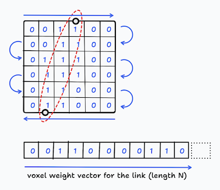
If we divide the entire environment, where the wireless network resides, into a grid, every unit square in this grid is called a voxel. The number of voxels we have depends on the number of rows and columns we break this field of network into. Let's depict the number of voxels as \(N\). Each link \(i\) spans cross a particular number of voxels in the grid. For a given link \(i\), the specific voxels that it goes through can be represented using a row vector \(w_{i}\) that has a length \(N\), i.e., the number of voxels. In this vector, the elements that are crossed by the link \(i\) are set 1, and the rest to 0. The following figure shows such a voxel weight vector created for a particular link.

Figure 2: Creating weight vector for a particular link.

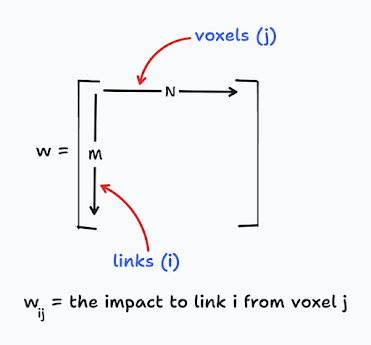
 We can create such a row vector \(w_{i}\) for each link \(i\). By doing so, we end up with \(M\) number such \(w_{i}\) row vectors. We can stack them together to create a matrix of weights. This matrix has a dimension of \(M \times N\) where \(M\) is the number of links and \(N\) is the number of voxels. The following figure illustrates how the combined weight matrix looks like. Using that matrix, we can refer to any particular link \(i\) impacted by a voxel \(j\) using the matrix element \(w_{ij}\). 

Figure 3: The resulting weight matrix that has weigh values for each link and each voxel.

Determining Shadowing Loss

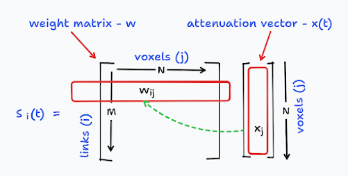
The shadowing loss, \({S}_{i}(t)\) is the sum of attenuation of the link \(i\) when it was going through the grid. Consider a column vector \(x(t)\) that has a length of \(N\), the number of voxels. Not all, but part of the voxels in the grid are crossed by the link \(i\). The attenuation of link \(i\) at a particular voxel \(j\) at time \(t\) is represented by the element \(x_{j}(t)\). Out of all elements in the \(x(t)\) vector, only the elements \(x_{j}(t)\) that have been crossed by the link \(i\) should be considered. We can find the relevance of an element in the vector \(x(t)\) for a link \(i\) by looking whether the corresponding value in the \(w_{ij}\) element of the weight matrix \(w\). If the corresponding element in the weight matrix is 1, that voxel's impact should be counted to the shadowing loss.

So, for particular link i, we can calculate it's shadowing loss in the following way, by using the weight matrix w and also the attenuation vector x.

$$ {S}_{i}(t) = \sum_{j=1}^{N} w_{ij} x_{j}(t) $$

It is important to note that we have to maintain consistency in the way we create the weight vector \(w_{i}\) and attenuation vector \(x\) for a given link \(i\) from its two dimensional matrix representation to a vector (see Figure 2).

The shadowing loss calculation can be visualised as follows:

Figure 4: Calculating shadowing loss for link \(i\) at time \(t\).

Changing Attenuation over Time

Due to the movement of obstacles, the received signal strength \({y}_{i}(t)\) varies over time. By focusing only on such changes, we can greatly simplify our mathematical representation. So, lets consider received signal values \({y}_{i}(t_{a})\) and \({y}_{i}(t_{b})\) for a link \(i\) at two times, \(t_{a}\) and \(t_{b}\). We can depict the difference of the received signal strengths \(\Delta y_{i}\) as follows:

$$ \Delta y_{i} = {y}_{i}(t_{b}) - {y}_{i}(t_{a}) $$

$$ \Delta y_{i} = \{ P_{i} - L_{i} - {S}_{i}(t_{b}) - {F}_{i}(t_{b}) - {\upsilon}_{i}(t_{b}) \} - \{ P_{i} - L_{i} - {S}_{i}(t_{a}) - {F}_{i}(t_{a}) - {\upsilon}_{i}(t_{a}) \} $$

$$ \Delta y_{i} = {S}_{i}(t_{a}) - {S}_{i}(t_{b}) + {F}_{i}(t_{a}) - {F}_{i}(t_{b}) + {\upsilon}_{i}(t_{a}) - {\upsilon}_{i}(t_{b}) $$ 

At this situation, we can consider the fading loss due to interferences, \({F}_{i}(t)\), and the measurement noise, \(\upsilon_{i}(t)\) altogether as an overall noise, \(n_{i}\) for the link \(i\) during the considered time period.  

$$ n_{i} = {F}_{i}(t_{a}) - {F}_{i}(t_{b}) + {\upsilon}_{i}(t_{a}) - {\upsilon}_{i}(t_{b}) $$

So, out equation for \(\Delta y_{i}\) can be rewritten as follows:

$$ \Delta y_{i} = {S}_{i}(t_{a}) - {S}_{i}(t_{b}) + n_{i} $$

Now, the difference between the two shadowing losses, \({S}_{i}(t_{a})\) and \({S}_{i}(t_{b})\), can also be closely inspected.

$$ {S}_{i}(t_{a}) - {S}_{i}(t_{b}) = \sum_{j=1}^{N} w_{ij} x_{j}(t_{a}) - \sum_{j=1}^{N} w_{ij} x_{j}(t_{b}) $$

$$ {S}_{i}(t_{a}) - {S}_{i}(t_{b}) = \sum_{j=1}^{N} w_{ij} \{(x_{j}(t_{a}) - x_{j}(t_{b})\} $$

$$ {S}_{i}(t_{a}) - {S}_{i}(t_{b}) = \sum_{j=1}^{N} w_{ij} \Delta x_{j} $$

So, we ended up with a new attenuation vector \(\Delta x_{j}\) that represents the variation of attenuation for the link \(i\). Considering that, we can further simplify our equation for the variation of received signal strength \(\Delta y_{i}\) as follows:

$$ \Delta y_{i} = \sum_{j=1}^{N} w_{ij} \Delta x_{j} + n_{i} $$

This equation that we finally ended up is really important. What it represents is the difference of the received signal strength of link \(i\) represented by \(\Delta y_{i}\). It can be calculated by using the weight matrix \(w\) and the difference of attenuation vector \(\Delta x\) for all the voxels from \(1\) to \(N\). 

There is a unique equation like this for each link \(i\) where \(i\) can be from \(1\) to \(M\).

$$ \Delta y_{1} = \sum_{j=1}^{N} w_{1j} \Delta x_{j} + n_{1} $$

$$ \Delta y_{2} = \sum_{j=1}^{N} w_{2j} \Delta x_{j} + n_{2} $$

$$ \Delta y_{3} = \sum_{j=1}^{N} w_{3j} \Delta x_{j} + n_{3} $$

$$ \ldots $$

$$ \Delta y_{M} = \sum_{j=1}^{N} w_{Mj} \Delta x_{j} + n_{M} $$

Let's represent this collection of equations (not linear equations) in the following format as a single equation:

$$ \Delta y = W \Delta x + n $$

Here, \(\Delta y\) is what we get to know that contains the variation of received signal strength for each link. By using that information, what we need to find is the \(\Delta x\) that contains a collection of attenuation vectors for each link. As a collective of these attenuation vectors, \(\Delta x\) represents the attenuation image (i.e., the tomographic image) that we need to create.